ANES96 — Multinomial logit on party identification
The 1996 American National Election Study records party
identification (PID) on a 7-point scale from strong Democrat (0)
to strong Republican (6), along with demographics and a 7-point
self-placed liberal-conservative scale (selfLR). Multinomial
logit on this kind of outcome is famously easy to fit and famously
easy to misreport — the coefficient table gives one log-odds
contrast per category against the baseline, and almost nobody
reading the paper will read it correctly.
pymargins handles MNL the same way it handles any other model:
ask for AMEs or predicted probabilities, and the result carries an
outcome axis you can slice.
This demo walks through:
Fit the MNL.
Predicted-probability profile across the ideology scale.
AMEs of ideology for each outcome category — the right way to report MNL effects.
A category-collapsed contrast (Democrat-leaning vs Republican-leaning) at a representative voter.
import numpy as np
import pandas as pd
import statsmodels.api as sm
import statsmodels.formula.api as smf

from pymargins import Margins

raw = sm.datasets.anes96.load_pandas().data.copy()
# 7-point PID coded 0..6. Keep covariates compact for the demo.
df = raw[["PID", "TVnews", "selfLR", "age", "educ", "income"]].dropna().copy()
df["PID"] = df["PID"].astype(int)
print(df.describe().round(2))
print("\nOutcome distribution:")
print(df["PID"].value_counts().sort_index())
          PID  TVnews  selfLR     age    educ  income
count  944.00  944.00  944.00  944.00  944.00  944.00
mean     2.84    3.73    4.33   47.04    4.57   16.33
std      2.27    2.68    1.44   16.42    1.60    5.97
min      0.00    0.00    1.00   19.00    1.00    1.00
25%      1.00    1.00    3.00   34.00    3.00   14.00
50%      2.00    3.00    4.00   44.00    4.00   17.00
75%      5.00    7.00    6.00   58.00    6.00   21.00
max      6.00    7.00    7.00   91.00    7.00   24.00

Outcome distribution:
PID
0    200
1    180
2    108
3     37
4     94
5    150
6    175
Name: count, dtype: int64
1. Fit the MNL
fit = smf.mnlogit(
    "PID ~ TVnews + selfLR + age + educ + income",
    data=df,
).fit(disp=False)
print(fit.summary().tables[1])
==============================================================================
     PID=1       coef    std err          z      P>|z|      [0.025      0.975]
------------------------------------------------------------------------------
Intercept     -0.2758      0.620     -0.445      0.656      -1.491       0.939
TVnews        -0.0994      0.043     -2.290      0.022      -0.185      -0.014
selfLR         0.2900      0.094      3.076      0.002       0.105       0.475
age           -0.0186      0.007     -2.619      0.009      -0.033      -0.005
educ           0.0808      0.073      1.100      0.271      -0.063       0.225
income         0.0041      0.018      0.233      0.815      -0.030       0.039
------------------------------------------------------------------------------
     PID=2       coef    std err          z      P>|z|      [0.025      0.975]
------------------------------------------------------------------------------
Intercept     -2.4823      0.750     -3.311      0.001      -3.952      -1.013
TVnews        -0.0368      0.050     -0.731      0.465      -0.136       0.062
selfLR         0.3901      0.108      3.616      0.000       0.179       0.602
age           -0.0201      0.009     -2.360      0.018      -0.037      -0.003
educ           0.1759      0.085      2.067      0.039       0.009       0.343
income         0.0502      0.022      2.270      0.023       0.007       0.093
------------------------------------------------------------------------------
     PID=3       coef    std err          z      P>|z|      [0.025      0.975]
------------------------------------------------------------------------------
Intercept     -3.8621      1.142     -3.383      0.001      -6.099      -1.625
TVnews        -0.0922      0.074     -1.238      0.216      -0.238       0.054
selfLR         0.5683      0.158      3.590      0.000       0.258       0.878
age           -0.0086      0.012     -0.699      0.484      -0.033       0.015
educ          -0.0154      0.127     -0.121      0.903      -0.263       0.233
income         0.0597      0.034      1.778      0.075      -0.006       0.126
------------------------------------------------------------------------------
     PID=4       coef    std err          z      P>|z|      [0.025      0.975]
------------------------------------------------------------------------------
Intercept     -7.7591      0.949     -8.178      0.000      -9.619      -5.900
TVnews        -0.0636      0.057     -1.126      0.260      -0.174       0.047
selfLR         1.2713      0.128      9.900      0.000       1.020       1.523
age           -0.0044      0.009     -0.480      0.631      -0.022       0.014
educ           0.1938      0.094      2.063      0.039       0.010       0.378
income         0.0849      0.026      3.261      0.001       0.034       0.136
------------------------------------------------------------------------------
     PID=5       coef    std err          z      P>|z|      [0.025      0.975]
------------------------------------------------------------------------------
Intercept     -7.2003      0.836     -8.612      0.000      -8.839      -5.562
TVnews        -0.0861      0.051     -1.696      0.090      -0.186       0.013
selfLR         1.3387      0.117     11.468      0.000       1.110       1.567
age           -0.0121      0.008     -1.454      0.146      -0.028       0.004
educ           0.2120      0.085      2.502      0.012       0.046       0.378
income         0.0812      0.023      3.554      0.000       0.036       0.126
------------------------------------------------------------------------------
     PID=6       coef    std err          z      P>|z|      [0.025      0.975]
------------------------------------------------------------------------------
Intercept    -12.3761      1.055    -11.735      0.000     -14.443     -10.309
TVnews        -0.0684      0.054     -1.266      0.205      -0.174       0.037
selfLR         2.0663      0.143     14.449      0.000       1.786       2.347
age           -0.0050      0.009     -0.563      0.573      -0.022       0.012
educ           0.3168      0.091      3.488      0.000       0.139       0.495
income         0.1101      0.025      4.379      0.000       0.061       0.159
==============================================================================
The coefficient table reports log-odds of each PID category against
the baseline (PID=0, strong Democrat). A coefficient of 0.5 on
selfLR for “PID=6” does not mean “0.5 percentage points more
likely to be a strong Republican” — it’s a log-odds contrast at a
covariate combination that may or may not exist in the data. This
is exactly why marginal-effects machinery exists.
2. Predicted probability profile across ideology
import matplotlib.pyplot as plt

m = Margins.linear_scale(fit, at="overall")
lr_grid = list(range(1, 8))  # selfLR scale 1..7
res = m.predict(atexog={"selfLR": lr_grid})

est = np.asarray(res.estimate)        # (n_lr, n_outcomes)
ci = np.asarray(res.conf_int())       # (2, n_lr, n_outcomes)
n_lr, n_out = est.shape

pid_labels = [
    "Strong Dem", "Weak Dem", "Ind-Dem",
    "Independent",
    "Ind-Rep", "Weak Rep", "Strong Rep",
]
# Blue = Democrat, red = Republican, grey = independent — standard US
# political color convention.
colors = ["#1f4e96", "#5588c8", "#a6c8e8",
          "#7f7f7f",
          "#e8a6a6", "#c85555", "#961f1f"]

fig, ax = plt.subplots(figsize=(7, 4))
for j in range(n_out):
    ax.plot(lr_grid, est[:, j], color=colors[j], label=pid_labels[j], lw=2)
    ax.fill_between(
        lr_grid, ci[0, :, j], ci[1, :, j], alpha=0.15, color=colors[j]
    )
ax.set(xlabel="Self-placed liberal–conservative (1=liberal, 7=conservative)",
       ylabel="P(PID category)",
       title="Predicted party-ID by ideology, sample-averaged")
ax.legend(loc="upper center", ncol=4, fontsize=8)
/home/hunter/Workspace/pymargins/pymargins/margins/_session.py:875: UserWarning: Delta-method curvature κ=0.533 exceeds threshold (0.3, stacklevel=2); falling back to simulation.
  result_data = run_inference(
<matplotlib.legend.Legend at 0x7f0b74fd6d20>
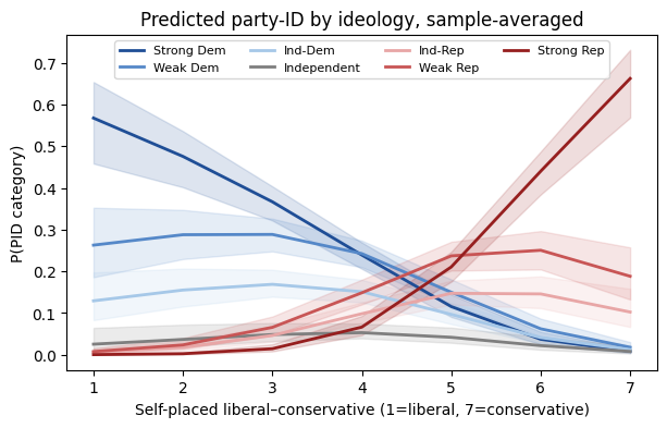
The crossover pattern — strong-Democrat probability falling, strong- Republican rising, with the middle categories peaking near the ideology center — is the kind of finding that becomes a figure in the paper. The coefficient table cannot give you this picture.
3. AME of ideology, per outcome category
The slope of selfLR is different for each PID category, because
the probabilities sum to 1 and a positive AME for one category
forces negative AMEs elsewhere:
ame_lr = m.dydx("selfLR")
print(ame_lr.summary())
/home/hunter/Workspace/pymargins/pymargins/margins/_session.py:972: UserWarning: Delta-method curvature κ=0.729 exceeds threshold (0.3, stacklevel=2); falling back to simulation.
  result_data = run_inference(
=================================================================
             Margins Result (simulation, level=0.95)
=================================================================
            estimate  std err  statistic  P>|z|  [95% Conf. Int.]
-----------------------------------------------------------------
selfLR (0)   -0.0967   0.0078    -0.0967  0.000  -0.1119, -0.0805
selfLR (1)   -0.0513   0.0072    -0.0513  0.000  -0.0663, -0.0378
selfLR (2)   -0.0274   0.0056    -0.0274  0.000  -0.0388, -0.0167
selfLR (3)   -0.0052   0.0034    -0.0052  0.052   -0.0132, 0.0000
selfLR (4)    0.0198   0.0054     0.0198  0.000    0.0099, 0.0307
selfLR (5)    0.0363   0.0068     0.0363  0.000    0.0237, 0.0503
selfLR (6)    0.1243   0.0084     0.1243  0.000    0.1082, 0.1411
=================================================================

n = 944
WARNING — Fallback triggered: kappa=0.729>threshold=0.3
κ: max=0.729
Each row of the result is the average per-unit change in the probability of that category, averaged across the sample. The columns sum to zero by construction (modulo numerical noise) — a sanity check that the AMEs are coherent.
The same for educ:
print(m.dydx("educ").summary())
/home/hunter/Workspace/pymargins/pymargins/margins/_session.py:972: UserWarning: Delta-method curvature κ=0.407 exceeds threshold (0.3, stacklevel=2); falling back to simulation.
  result_data = run_inference(
===============================================================
            Margins Result (simulation, level=0.95)
===============================================================
          estimate  std err  statistic  P>|z|  [95% Conf. Int.]
---------------------------------------------------------------
educ (0)   -0.0197   0.0084    -0.0197  0.021  -0.0361, -0.0031
educ (1)   -0.0054   0.0084    -0.0054  0.509   -0.0220, 0.0113
educ (2)    0.0065   0.0070     0.0065  0.353   -0.0072, 0.0205
educ (3)   -0.0056   0.0048    -0.0056  0.193   -0.0158, 0.0031
educ (4)    0.0016   0.0067     0.0016  0.807   -0.0114, 0.0148
educ (5)    0.0051   0.0079     0.0051  0.546   -0.0108, 0.0203
educ (6)    0.0174   0.0075     0.0174  0.014    0.0031, 0.0322
===============================================================

n = 944
WARNING — Fallback triggered: kappa=0.407>threshold=0.3
κ: max=0.407
4. Collapsed contrast — Democrat-leaning vs Republican-leaning
For a “headline number” you often want to collapse PID categories into two camps. The cleanest way is to build a custom estimand that wraps the predicted-probability vector:
import jax.numpy as jnp

def dem_minus_rep(p):
    # p: (n_scenarios, n_outcomes=7) — per-scenario category probabilities.
    # Returns one gap per scenario.
    dem = p[..., 0:3].sum(axis=-1)   # strong Dem, weak Dem, ind-Dem
    rep = p[..., 4:7].sum(axis=-1)   # ind-Rep, weak Rep, strong Rep
    return dem - rep

# One scenario per ideology level; compose collapses the outcome axis.
scenarios = [{"atexog": {"selfLR": v}, "label": f"selfLR={v}"}
             for v in lr_grid]
res_diff = m.evaluate(scenarios=scenarios, compose=dem_minus_rep)
print(res_diff.summary())
/home/hunter/Workspace/pymargins/pymargins/margins/_session.py:1345: UserWarning: Delta-method curvature κ=0.336 exceeds threshold (0.3, stacklevel=2); falling back to simulation.
  result_data = run_inference(
===================================================================
              Margins Result (simulation, level=0.95)
===================================================================
              estimate  std err  statistic  P>|z|  [95% Conf. Int.]
-------------------------------------------------------------------
selfLR=1 (0)    0.9461   0.0173     0.9461  0.000    0.9004, 0.9669
selfLR=1 (1)    0.8752   0.0236     0.8752  0.000    0.8152, 0.9088
selfLR=1 (2)    0.6979   0.0331     0.6979  0.000    0.6206, 0.7513
selfLR=1 (3)    0.3196   0.0379     0.3196  0.000    0.2387, 0.3868
selfLR=1 (4)   -0.2329   0.0414    -0.2329  0.000  -0.3118, -0.1496
selfLR=1 (5)   -0.6961   0.0367    -0.6961  0.000  -0.7566, -0.6138
selfLR=1 (6)   -0.9153   0.0196    -0.9153  0.000  -0.9427, -0.8680
===================================================================

n = 944
WARNING — Fallback triggered: kappa=0.336>threshold=0.3
κ: max=0.336
The result is the gap (P(Democrat-leaning) − P(Republican-leaning)) at each ideology level, with delta-method standard errors propagated through both the MNL link and the category sum. That single number is what most write-ups actually need.
Where to next
Multinomial logit — the underlying multinomial-logit tutorial.
Nonlinear estimands with evaluate —
evaluatefor custom estimands.Linear contrasts with contrasts — built-in contrast helpers for the common pairwise / reference / pooled patterns.