GLM — Binomial logit

A logit with factor variables and an interaction, every Stata margins analysis side-by-side with the pymargins call that produces it.

import numpy as np
import pandas as pd
import statsmodels.api as sm
import statsmodels.formula.api as smf

from pymargins import Margins

rng = np.random.default_rng(42)
n = 5000
female = rng.binomial(1, 0.52, n)
black = rng.binomial(1, 0.11, n)
age = rng.integers(20, 75, n)
agegrp = pd.cut(age, bins=[19, 29, 39, 49, 59, 69, 100],
                labels=[1, 2, 3, 4, 5, 6]).astype(int)
bmi = np.clip(22 + 0.15 * age + 1.5 * female + rng.normal(0, 4, n), 15, 50)
lp = (-4.0 + 0.55 * black + 0.10 * female + 0.06 * age + 0.03 * bmi
      + 0.5 * (agegrp == 2) + 0.9 * (agegrp == 3)
      + 1.4 * (agegrp == 4) + 2.0 * (agegrp == 5) + 2.6 * (agegrp == 6))
df = pd.DataFrame({
    "diabetes": rng.binomial(1, 1 / (1 + np.exp(-lp))),
    "black": black, "female": female, "age": age, "agegrp": agegrp, "bmi": bmi,
})

fit = smf.glm(
    "diabetes ~ C(black) + C(female) + C(agegrp) + bmi + age",
    data=df,
    family=sm.families.Binomial(),
).fit()

APM — predictions at the typical profile

Stata: margins agegrp, atmeans.

For predicted probabilities the natural reporting scale is the probability scale itself, so linear_scale is the default that matches Stata:

print(Margins.linear_scale(fit, at="typical").predict(
    atexog={"agegrp": list(range(1, 7))}
).summary())

===============================================================
            Margins Result (simulation, level=0.95)            
===============================================================
          estimate  std err  statistic  P>|z|  [95% Conf. Int.]
---------------------------------------------------------------
agegrp=1    0.5121   0.0737     0.5121  0.000    0.3639, 0.6546
agegrp=2    0.5950   0.0431     0.5950  0.000    0.5086, 0.6766
agegrp=3    0.6575   0.0189     0.6575  0.000    0.6183, 0.6941
agegrp=4    0.7388   0.0261     0.7388  0.000    0.6847, 0.7866
agegrp=5    0.8062   0.0416     0.8062  0.000    0.7119, 0.8735
agegrp=6    0.9566   0.0362     0.9566  0.000    0.8529, 0.9881
===============================================================

n = 5000
WARNING — Fallback triggered: kappa=0.607>threshold=0.3
κ: max=0.607

/home/hunter/Workspace/pymargins/pymargins/margins/_session.py:704: UserWarning: Delta-method curvature κ=0.607 exceeds threshold (0.3); falling back to simulation.
  result_data = run_inference(

AAP — averaged over the sample

Stata: margins agegrp.

print(Margins.linear_scale(fit, at="overall").predict(
    atexog={"agegrp": list(range(1, 7))}
).summary())

/home/hunter/Workspace/pymargins/pymargins/margins/_session.py:704: UserWarning: Delta-method curvature κ=0.531 exceeds threshold (0.3); falling back to simulation.
  result_data = run_inference(

===============================================================
            Margins Result (simulation, level=0.95)            
===============================================================
          estimate  std err  statistic  P>|z|  [95% Conf. Int.]
---------------------------------------------------------------
agegrp=1    0.5152   0.0551     0.5152  0.000    0.3919, 0.6100
agegrp=2    0.5770   0.0273     0.5770  0.000    0.5164, 0.6210
agegrp=3    0.6251   0.0123     0.6251  0.000    0.6012, 0.6487
agegrp=4    0.6915   0.0317     0.6915  0.000    0.6312, 0.7541
agegrp=5    0.7521   0.0508     0.7521  0.000    0.6483, 0.8464
agegrp=6    0.9272   0.0513     0.9272  0.000    0.7903, 0.9822
===============================================================

n = 5000
WARNING — Fallback triggered: kappa=0.531>threshold=0.3
κ: max=0.531

APR — at representative values

Stata: margins, at(age=(20 50 70)) atmeans.

print(Margins.linear_scale(fit, at="typical").predict(
    atexog={"age": [20, 50, 70]}
).summary())

===========================================================
             Margins Result (delta, level=0.95)            
===========================================================
        estimate  std err        z  P>|z|  [95% Conf. Int.]
-----------------------------------------------------------
age=20    0.2079   0.0539   3.8549  0.000    0.1022, 0.3136
age=50    0.7054   0.0221  31.9227  0.000    0.6621, 0.7487
age=70    0.9127   0.0272  33.5007  0.000    0.8593, 0.9661
===========================================================

n = 5000
κ: max=0.282
Delta-vs-sim disagreement: 10.421%

MEM and AME

Stata: margins, dydx(age) atmeans and margins, dydx(age).

Margins.linear_scale(fit, at="typical").dydx("age").summary()
print(Margins.linear_scale(fit, at="overall").dydx("age").summary())

=======================================================
           Margins Result (delta, level=0.95)          
=======================================================
     estimate  std err       z  P>|z|  [95% Conf. Int.]
-------------------------------------------------------
age    0.0106   0.0025  4.2317  0.000    0.0057, 0.0155
=======================================================

n = 5000
κ: 0.015
Delta-vs-sim disagreement: 12.918%

Discrete change

For binary regressors, dydx is a derivative — the discrete change on the response scale is a contrast across the two levels:

from pymargins import pairwise

scen, w = pairwise("black", [1, 0])
print(Margins.linear_scale(fit, at="overall").contrasts(
    scenarios=scen, contrasts=w
).summary())

===========================================================
             Margins Result (delta, level=0.95)            
===========================================================
         estimate  std err       z  P>|z|  [95% Conf. Int.]
-----------------------------------------------------------
black=1    0.0870   0.0167  5.1965  0.000    0.0542, 0.1198
===========================================================

n = 5000
κ: 0.027
Delta-vs-sim disagreement: 2.040%

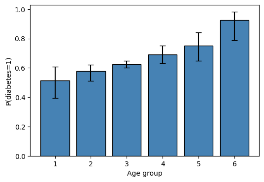
Plot: predicted probability by age group

import matplotlib.pyplot as plt

res = Margins.linear_scale(fit, at="overall").predict(
    atexog={"agegrp": list(range(1, 7))}
)
df_plot = res.to_frame()

fig, ax = plt.subplots(figsize=(6, 4))
ax.bar(df_plot["agegrp"].astype(str), df_plot["estimate"],
       yerr=[df_plot["estimate"] - df_plot["ci_lower"],
             df_plot["ci_upper"] - df_plot["estimate"]],
       capsize=4, color="steelblue", edgecolor="black")
ax.set(xlabel="Age group", ylabel="P(diabetes=1)")

/home/hunter/Workspace/pymargins/pymargins/margins/_session.py:704: UserWarning: Delta-method curvature κ=0.531 exceeds threshold (0.3); falling back to simulation.
  result_data = run_inference(

[Text(0.5, 0, 'Age group'), Text(0, 0.5, 'P(diabetes=1)')]

Robust SEs

print(Margins.linear_scale(fit, vcov="HC3", at="overall").dydx("age").summary())

=======================================================
           Margins Result (delta, level=0.95)          
=======================================================
     estimate  std err       z  P>|z|  [95% Conf. Int.]
-------------------------------------------------------
age    0.0106   0.0025  4.2620  0.000    0.0057, 0.0155
=======================================================

n = 5000
κ: 0.015
Delta-vs-sim disagreement: 13.485%