Per-observation influence

MarginsResult.influence() returns, for each training observation, how much that observation contributes to the estimate — the leave-one-out deletion influence θ̂ − θ_{(-i)}. Unlike statsmodels’ built-in influence diagnostics (which describe the coefficients β), this works for the estimand you actually report: an average marginal effect, a contrast, an elasticity, an RMST. A large positive value means dropping that observation would pull the estimate down.

import numpy as np
import pandas as pd
import statsmodels.api as sm
import statsmodels.formula.api as smf
from pymargins import Margins

rng = np.random.default_rng(1)
n = 180
df = pd.DataFrame({
    "x": rng.normal(0, 1, n),
    "z": rng.normal(0, 1, n),
})
lp = -0.5 + 0.8 * df["x"] - 0.4 * df["z"]
df["y"] = rng.binomial(1, 1 / (1 + np.exp(-lp)))

fit = smf.glm("y ~ x + z", data=df, family=sm.families.Binomial()).fit()
m = Margins.linear_scale(fit, at="overall")

ame = m.dydx("x")
print(ame.summary())

=====================================================
          Margins Result (delta, level=0.95)         
=====================================================
   estimate  std err       z  P>|z|  [95% Conf. Int.]
-----------------------------------------------------
x    0.1761   0.0360  4.8954  0.000    0.1056, 0.2467
=====================================================

n = 180
κ: 0.124
Delta-vs-sim disagreement: 4.533%

Basic usage

infl = ame.influence()
infl.shape          # (n_obs,) for a scalar estimand

(180,)

The values are signed and (to first order) sum to zero, since the score contributions cancel at the fitted estimate:

print("sum of influence ≈", float(infl.sum()))

sum of influence ≈ 5.204170427930421e-17

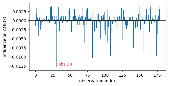
Finding the most influential observations

Sort by absolute influence to see which rows move the marginal effect most — a Cook’s-distance analogue, but for the AME rather than the coefficients.

order = np.argsort(-np.abs(infl))
top = df.iloc[order[:5]].copy()
top["influence"] = infl[order[:5]]
print(top)

            x         z  y  influence
30   2.117839  0.501483  0  -0.012894
82  -1.630849 -1.760329  1  -0.010275
108  1.753384 -1.392102  0  -0.009794
174 -1.670850  0.873416  1  -0.009776
155  1.627300 -0.030583  0  -0.008954

Reconstructing the variance

Summing the squared influence reconstructs the robust (HC0) sandwich variance of the estimand — because Σ_i score_i score_iᵀ is exactly the sandwich “meat”:

se_from_influence = np.sqrt(np.sum(infl ** 2))

m_hc0 = Margins.linear_scale(fit, at="overall", vcov="HC0")
se_hc0 = float(np.atleast_1d(m_hc0.dydx("x").std_error)[0])

print(f"sqrt(Σ influence²) = {se_from_influence:.6f}")
print(f"HC0 robust SE      = {se_hc0:.6f}")

sqrt(Σ influence²) = 0.036726
HC0 robust SE      = 0.036726

The two agree to numerical precision. (The default model-based SE differs because it assumes the information equality holds in-sample.) Summing influence within clusters before squaring gives the cluster-robust variance — the same construction at a coarser grouping.

Two routes, same quantity

The example above uses the delta method: the analytical influence function ∇h(β̂)ᵀ Σ̂ score_i(β̂), where Σ̂ score_i is the one-step (infinitesimal jackknife) approximation to β̂ − β̂_{(-i)}.

A BCa bootstrap result returns the exact leave-one-out refits that were already computed for the acceleration constant — no extra work:

m_boot = Margins.linear_scale(
    fit, at="overall", method="bootstrap",
    n_boot=200, rng_seed=0,
    bootstrap_config={"ci_method": "bca"},
)
infl_jack = m_boot.dydx("x").influence()

corr = np.corrcoef(infl, infl_jack)[0, 1]
print(f"correlation(delta, jackknife) = {corr:.4f}")

correlation(delta, jackknife) = 0.9525

The two are strongly correlated. They are not identical: the delta route is a one-step approximation, so it differs from the exact refit by the leverage factor 1/(1 − h_ii) and, for a nonlinear estimand like a logit AME, by higher-order curvature. The delta route is far cheaper (no refits) and has no sample-size cap; the jackknife is exact but limited (see pitfalls).

Vector estimands

For a length-k vector result (e.g. a prediction over several scenarios), influence() returns an (n_obs, k) matrix — one influence column per component:

r_vec = m.predict(atexog={"x": [-1.0, 0.0, 1.0]})
infl_vec = r_vec.influence()
infl_vec.shape

(180, 3)

Plot: an influence index plot

import matplotlib.pyplot as plt

fig, ax = plt.subplots(figsize=(6, 3))
ax.stem(np.arange(n), infl, markerfmt=" ", basefmt="C7-")
ax.axhline(0, color="black", lw=0.8)
ax.set(xlabel="observation index", ylabel="influence on AME(x)")
top_i = order[0]
ax.annotate(f"obs {top_i}", (top_i, infl[top_i]),
            textcoords="offset points", xytext=(5, 5), color="C3")

Text(5, 5, 'obs 30')

Which models support it

The delta-method route needs per-observation scores via adapter.score_obs(). This is implemented for the statsmodels GLM (all families/links), OLS, Logit/Probit, and Poisson/NegativeBinomial adapters. Adapters without score_obs() raise NotImplementedError on the delta route — but the BCa bootstrap route works for any bootstrappable model.

Pitfalls

• Keep the session alive. The delta route reads scores from the live adapter, so the Margins session must still be in scope: m.dydx("x").influence() works, but Margins.linear_scale(fit).dydx("x").influence() may fail if the session is garbage-collected first. Materialized results (which drop the session) cannot use the delta route.

• Jackknife size cap. The BCa leave-one-out refits are skipped when n_obs (or the number of clusters) exceeds 200, and for block bootstrap where leave-one-out is not well defined. In those cases use the delta route, which has no size limit.

• vcov changes the meaning. Influence is formed with the session’s frozen Σ̂. Under a robust or cluster vcov it becomes the corresponding sandwich influence rather than the model-based one — usually what you want, but worth stating in a write-up.