Rossi recidivism — Cox proportional hazards end-to-end

The Rossi data tracks 432 male convicts released from Maryland state prisons in the 1970s for up to 52 weeks. The outcome is time to first re-arrest; the censoring indicator is arrest. The substantive question is whether a randomly assigned financial-aid intervention (fin) reduced recidivism, controlling for age, race, prior work experience, marital status, parole status, and prior convictions.

This demo runs the analysis the way you’d want to publish it:

1. Fit a Cox PH model.

2. Marginal log hazard ratio for the financial-aid treatment.

3. Subgroup treatment effect across prio (number of prior convictions).

4. Predicted survival curves at representative profiles.

5. A bootstrap cross-check on the treatment effect.

import numpy as np
import pandas as pd
from lifelines import CoxPHFitter
from lifelines.datasets import load_rossi

from pymargins import Margins, pairwise
from pymargins.adapters import LifelinesCoxPHAdapter

df = load_rossi()
print(df.head())
print(f"\nn = {len(df)}, events = {df['arrest'].sum()}, "
      f"max follow-up = {df['week'].max()} weeks")

   week  arrest  fin  age  race  wexp  mar  paro  prio
0    20       1    0   27     1     0    0     1     3
1    17       1    0   18     1     0    0     1     8
2    25       1    0   19     0     1    0     1    13
3    52       0    1   23     1     1    1     1     1
4    52       0    0   19     0     1    0     1     3

n = 432, events = 114, max follow-up = 52 weeks

1. Fit the Cox PH model

cph = CoxPHFitter().fit(df, duration_col="week", event_col="arrest")
print(cph.summary[["coef", "exp(coef)", "se(coef)", "p"]].round(3))

            coef  exp(coef)  se(coef)      p
covariate                                   
fin       -0.379      0.684     0.191  0.047
age       -0.057      0.944     0.022  0.009
race       0.314      1.369     0.308  0.308
wexp      -0.150      0.861     0.212  0.480
mar       -0.434      0.648     0.382  0.256
paro      -0.085      0.919     0.196  0.665
prio       0.091      1.096     0.029  0.001

The raw fin coefficient is the log hazard ratio for treatment under Cox’s partial likelihood — but coefficient tables don’t average over the sample’s covariate distribution. That’s what the Margins session is for.

2. Marginal treatment effect on the log-hazard scale

Cox is multiplicative, so the natural inference scale is log:

adapter = LifelinesCoxPHAdapter(cph, training_data=df)
m = Margins.log_scale(cph, adapter=adapter, at="overall")

scen, w = pairwise("fin", [1, 0])
hr = m.contrasts(scenarios=scen, contrasts=w)
print(hr.summary())

==========================================================
            Margins Result (delta, level=0.95)            
==========================================================
       estimate  std err        z  P>|z|  [95% Conf. Int.]
----------------------------------------------------------
fin=1    0.6843   0.1914  -1.9826  0.047    0.4702, 0.9957
==========================================================

n = 432
Note: std err is on the inference scale; estimate and CI are on the reporting scale.
κ: 0.000
Delta-vs-sim disagreement: 2.087%

The point estimate is the population-averaged log hazard ratio for financial aid; the back-transformed interval is the hazard ratio with asymmetric CI. For a Cox model the AAP-style averaging coincides with the raw coefficient (the partial likelihood is invariant to non-treatment covariates by design), so the value reported here will match cph.summary.loc["fin"] — but the session machinery now extends to derived quantities the summary table cannot give you, as the next two sections show.

3. Does the effect depend on prior convictions?

prio is a count regressor recording prior convictions. To check whether the treatment is more or less helpful for repeat offenders, ask for the treatment contrast at several representative prio levels at once:

prio_levels = [0, 2, 4, 6]
k = len(prio_levels)
scenarios = (
    [{"atexog": {"fin": 1, "prio": p},
      "label": f"fin=1, prio={p}"} for p in prio_levels]
    + [{"atexog": {"fin": 0, "prio": p},
        "label": f"fin=0, prio={p}"} for p in prio_levels]
)
W = np.zeros((k, 2 * k))
for i in range(k):
    W[i, i] = +1.0
    W[i, k + i] = -1.0
het = m.contrasts(scenarios=scenarios, contrasts=W)
print(het.summary())

================================================================
               Margins Result (delta, level=0.95)               
================================================================
             estimate  std err        z  P>|z|  [95% Conf. Int.]
----------------------------------------------------------------
contrast[0]    0.6843   0.1914  -1.9826  0.047    0.4702, 0.9957
contrast[1]    0.6843   0.1914  -1.9826  0.047    0.4702, 0.9957
contrast[2]    0.6843   0.1914  -1.9826  0.047    0.4702, 0.9957
contrast[3]    0.6843   0.1914  -1.9826  0.047    0.4702, 0.9957
================================================================

n = 432
Note: std err is on the inference scale; estimate and CI are on the reporting scale.
κ: max=0.000
Delta-vs-sim disagreement: 1.876%

Under proportional hazards the log HR for fin is constant in prio by construction — so this table is also a sanity check on the PH assumption: if the per-level effects drift, the proportionality assumption is suspect. (For real-world non-PH effects you would fit a stratified or time-varying model first; the same session API works against either.)

4. Hazard-ratio profile across age

The session-API equivalent of a “forest plot across age” is a sweep of the treatment contrast at fixed age values. Each row is the treatment effect (fin=1 vs fin=0) for someone of that age, with every other covariate held at its observed sample distribution:

import matplotlib.pyplot as plt

ages = list(range(18, 51, 4))
n = len(ages)
scenarios = (
    [{"atexog": {"fin": 1, "age": a}, "label": f"fin=1, age={a}"} for a in ages]
    + [{"atexog": {"fin": 0, "age": a}, "label": f"fin=0, age={a}"} for a in ages]
)
# One contrast per age: +1 on treated row, -1 on the matching control row.
W = np.zeros((n, 2 * n))
for i in range(n):
    W[i, i] = +1.0
    W[i, n + i] = -1.0
res_age = m.contrasts(scenarios=scenarios, contrasts=W)
df_age = res_age.to_frame()
df_age["age"] = ages

fig, ax = plt.subplots(figsize=(6, 4))
ax.plot(df_age["age"], df_age["estimate"], "o-", color="firebrick")
ax.fill_between(
    df_age["age"], df_age["ci_lower"], df_age["ci_upper"],
    alpha=0.2, color="firebrick",
)
ax.axhline(1.0, color="grey", lw=0.5)
ax.set(xlabel="Age at release",
       ylabel="Treatment hazard ratio (fin=1 vs fin=0)")

[Text(0.5, 0, 'Age at release'),
 Text(0, 0.5, 'Treatment hazard ratio (fin=1 vs fin=0)')]

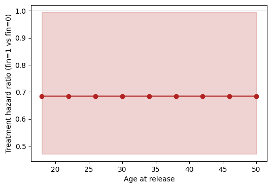
Under proportional hazards the hazard ratio is constant in age by construction. If the curve drifts materially with age, the PH assumption is suspect — a useful visual diagnostic of the model in addition to a presentation of the estimand.

5. Bootstrap cross-check

Cox partial likelihood inference is reliable in the central case; the bootstrap is still useful when you want a sanity check that doesn’t depend on the partial-likelihood asymptotics:

m_boot = Margins.log_scale(
    cph, adapter=adapter, at="overall",
    method="bootstrap", n_boot=300, rng_seed=0,
)
print(m_boot.contrasts(scenarios=scen, contrasts=w).summary())

============================================================
           Margins Result (bootstrap, level=0.95)           
============================================================
       estimate  std err  statistic  P>|z|  [95% Conf. Int.]
------------------------------------------------------------
fin=1    0.6843   0.2039    -0.3794  0.053    0.4697, 0.9944
============================================================

n = 432
Note: std err is on the inference scale; estimate and CI are on the reporting scale.
κ: 0.000

For this sample size and event count the bootstrap CI agrees closely with the partial-likelihood CI from §2 — exactly the boring result you want.

6. Counterfactual survival curves

The hazard-ratio analyses above answer “does the treatment change the relative re-arrest rate.” A reviewer reading the paper will also want the absolute survival curve under each treatment arm, standardized over the sample. That’s the pymargins analogue of a Kaplan–Meier plot for the counterfactual fin=1 vs fin=0 worlds, adjusted for the rest of the covariates.

Each scenario carries its own prediction_time; one bootstrap pass covers the entire grid because the refit cache is session-level.

from pymargins.adapters import LifelinesCoxPHSurvivalAdapter

surv_adapter = LifelinesCoxPHSurvivalAdapter(cph, training_data=df)
m_surv = Margins(
    cph, adapter=surv_adapter, at="overall",
    method="bootstrap", n_boot=300, rng_seed=0,
)

weeks = np.arange(4, 53, 4)
scens = (
    [{"atexog": {"fin": 1}, "prediction_time": float(t),
      "label": f"fin=1,t={t}"} for t in weeks]
    + [{"atexog": {"fin": 0}, "prediction_time": float(t),
        "label": f"fin=0,t={t}"} for t in weeks]
)
curves = m_surv.contrasts(scenarios=scens, contrasts=np.eye(len(scens)))
curve_df = curves.to_frame()
curve_df["arm"] = ["fin=1"] * len(weeks) + ["fin=0"] * len(weeks)
curve_df["week"] = list(weeks) * 2

fig, ax = plt.subplots(figsize=(6, 4))
for arm, color in [("fin=0", "steelblue"), ("fin=1", "firebrick")]:
    sub = curve_df[curve_df["arm"] == arm]
    ax.plot(sub["week"], sub["estimate"], "-o", color=color, label=arm)
    ax.fill_between(sub["week"], sub["ci_lower"], sub["ci_upper"],
                    alpha=0.15, color=color)
ax.set(xlabel="Week", ylabel="Counterfactual survival probability",
       ylim=(0.5, 1.0))
ax.legend()

<matplotlib.legend.Legend at 0x7f3518ee9dc0>

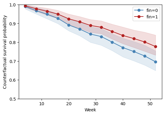
The bands are bootstrap percentile intervals, computed jointly across treatment arms and times because every estimand in this session shares the same resample bank.

The difference curve S₁(t) − S₀(t) is a contrast over the same scenarios — one row of weights per week, +1 on the treated atom and −1 on the matched control atom:

k = len(weeks)
W = np.zeros((k, 2 * k))
for i in range(k):
    W[i, i] = +1.0       # treated arm at week i
    W[i, k + i] = -1.0   # control arm at the same week
diff = m_surv.contrasts(scenarios=scens, contrasts=W)
diff_df = diff.to_frame()
diff_df["week"] = list(weeks)

fig, ax = plt.subplots(figsize=(6, 4))
ax.plot(diff_df["week"], diff_df["estimate"], "-o", color="black")
ax.fill_between(diff_df["week"], diff_df["ci_lower"], diff_df["ci_upper"],
                alpha=0.2, color="black")
ax.axhline(0.0, color="grey", lw=0.5)
ax.set(xlabel="Week", ylabel="S(t | fin=1) − S(t | fin=0)")

[Text(0.5, 0, 'Week'), Text(0, 0.5, 'S(t | fin=1) − S(t | fin=0)')]

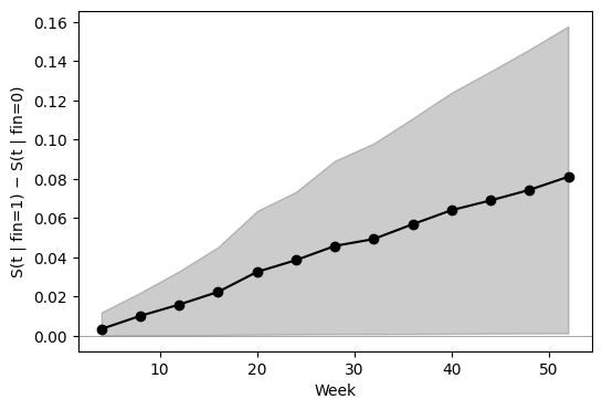
Because both curves came from the same Margins session, their draws_inf are aligned per replicate — the difference is a valid bootstrap estimand without extra reweighting.

Where to next

• Cox proportional hazards — the underlying Cox tutorial.

• Accelerated failure time models — parametric survival, where the natural inference scale is time rather than hazard.

• The adapter pattern — how the lifelines adapter exposes hazard- and survival-scale estimands behind the same session API.