Mroz (1987) — Female labor force participation
The Mroz data is the canonical textbook example for a binary-choice
labor model: 753 married women observed in 1975, with a binary
indicator inlf for whether they participated in the labor force.
The covariates are family non-wife income, education, experience
(plus its square), age, and counts of young (kidslt6) and older
(kidsge6) children.
This demo runs a complete pymargins analysis end-to-end:
Fit a logit.
Compare AMEs vs MEMs — the canonical case where they materially differ.
Discrete-change effect of an additional young child.
Predicted participation curve over education, by number of young children.
A bootstrap confidence interval on the discrete-change effect for comparison with the delta-method result.
import numpy as np
import pandas as pd
import statsmodels.api as sm
import statsmodels.formula.api as smf
from linearmodels.datasets import mroz

from pymargins import Margins, pairwise

cols = ["inlf", "nwifeinc", "educ", "exper", "age", "kidslt6", "kidsge6"]
df = mroz.load()[cols].dropna().copy()
df["expersq"] = df["exper"] ** 2
print(df.describe().round(2))
         inlf  nwifeinc    educ   exper     age  kidslt6  kidsge6  expersq
count  753.00    753.00  753.00  753.00  753.00   753.00   753.00   753.00
mean     0.57     20.13   12.29   10.63   42.54     0.24     1.35   178.04
std      0.50     11.63    2.28    8.07    8.07     0.52     1.32   249.63
min      0.00      0.03    5.00    0.00   30.00     0.00     0.00     0.00
25%      0.00     13.03   12.00    4.00   36.00     0.00     0.00    16.00
50%      1.00     17.70   12.00    9.00   43.00     0.00     1.00    81.00
75%      1.00     24.47   13.00   15.00   49.00     0.00     2.00   225.00
max      1.00     96.00   17.00   45.00   60.00     3.00     8.00  2025.00
1. Fit the participation logit
fit = smf.glm(
    "inlf ~ nwifeinc + educ + exper + expersq + age + kidslt6 + kidsge6",
    data=df,
    family=sm.families.Binomial(),
).fit()
print(fit.summary().tables[1])
==============================================================================
                 coef    std err          z      P>|z|      [0.025      0.975]
------------------------------------------------------------------------------
Intercept      0.4255      0.860      0.495      0.621      -1.261       2.112
nwifeinc      -0.0213      0.008     -2.535      0.011      -0.038      -0.005
educ           0.2212      0.043      5.091      0.000       0.136       0.306
exper          0.2059      0.032      6.422      0.000       0.143       0.269
expersq       -0.0032      0.001     -3.104      0.002      -0.005      -0.001
age           -0.0880      0.015     -6.040      0.000      -0.117      -0.059
kidslt6       -1.4434      0.204     -7.090      0.000      -1.842      -1.044
kidsge6        0.0601      0.075      0.804      0.422      -0.086       0.207
==============================================================================
2. AME vs MEM — why the choice matters
The marginal effect of education on P(inlf=1) is nonlinear in the linear predictor, so the average of per-row effects (AME) is not the same as the effect evaluated at the sample mean profile (MEM). For a participation rate near 0.5 the two are usually close; for rates near 0 or 1 they can disagree by an order of magnitude.
m_ame = Margins.linear_scale(fit, vcov="HC3", at="overall")
m_mem = Margins.linear_scale(fit, vcov="HC3", at="typical")

print("AME (averaged over sample):")
print(m_ame.dydx("educ").summary())
print("\nMEM (at the typical profile):")
print(m_mem.dydx("educ").summary())
AME (averaged over sample):
========================================================
           Margins Result (delta, level=0.95)
========================================================
      estimate  std err       z  P>|z|  [95% Conf. Int.]
--------------------------------------------------------
educ    0.0410   0.0074  5.5788  0.000    0.0266, 0.0555
========================================================

n = 753
κ: 0.051
Delta-vs-sim disagreement: 3.666%

MEM (at the typical profile):
========================================================
           Margins Result (delta, level=0.95)
========================================================
      estimate  std err       z  P>|z|  [95% Conf. Int.]
--------------------------------------------------------
educ    0.0571   0.0109  5.2543  0.000    0.0358, 0.0784
========================================================

n = 753
κ: 0.046
Delta-vs-sim disagreement: 10.524%
The AME for educ here is the right number to report in a paper;
the MEM exists for replication of Stata atmeans output.
3. Discrete change — one additional child under six
kidslt6 is a count regressor, but for policy interpretation the
quantity of interest is the effect of having one more young child,
not the partial derivative. That’s a contrast, not a slope:
scen, w = pairwise("kidslt6", [1, 0])
delta = m_ame.contrasts(scenarios=scen, contrasts=w)
print(delta.summary())
==============================================================
              Margins Result (delta, level=0.95)
==============================================================
           estimate  std err        z  P>|z|  [95% Conf. Int.]
--------------------------------------------------------------
kidslt6=1   -0.2697   0.0351  -7.6782  0.000  -0.3386, -0.2009
==============================================================

n = 753
κ: 0.056
Delta-vs-sim disagreement: 2.195%
The estimate is the population-average drop in participation
probability associated with moving from zero to one young child,
holding every other covariate at its observed value. Compare to the
naive dydx("kidslt6"):
print(m_ame.dydx("kidslt6").summary())
=============================================================
              Margins Result (delta, level=0.95)
=============================================================
         estimate  std err         z  P>|z|  [95% Conf. Int.]
-------------------------------------------------------------
kidslt6   -0.2573   0.0216  -11.9238  0.000  -0.2996, -0.2150
=============================================================

n = 753
κ: 0.260
Delta-vs-sim disagreement: 11.935%
The two answer different questions. The derivative assumes a smooth treatment intensity that doesn’t exist; the contrast is what an audience usually wants.
4. Education profile by family composition
import matplotlib.pyplot as plt

educ_grid = list(range(5, 18))
res = m_ame.predict(atexog={"educ": educ_grid, "kidslt6": [0, 1, 2]})
df_plot = res.to_frame()

fig, ax = plt.subplots(figsize=(6, 4))
for k, sub in df_plot.groupby("kidslt6"):
    ax.plot(sub["educ"], sub["estimate"], label=f"{k} young child(ren)")
    ax.fill_between(
        sub["educ"], sub["ci_lower"], sub["ci_upper"], alpha=0.15
    )
ax.set(xlabel="Years of education",
       ylabel="P(in labor force)",
       title="Predicted participation, averaged over other covariates")
ax.legend()
/home/hunter/Workspace/pymargins/pymargins/margins/_session.py:875: UserWarning: Delta-method curvature κ=0.454 exceeds threshold (0.3, stacklevel=2); falling back to simulation.
  result_data = run_inference(
<matplotlib.legend.Legend at 0x7fbf34429100>
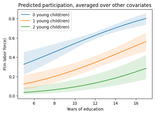
Two things show up immediately on this plot that you cannot read off the coefficient table: the slope of education flattens as kids under six accumulate, and the gap between the kid-curves is widest at intermediate education — both implications of the logit link, not of any new parameter.
5. Bootstrap cross-check on the discrete change
The session API lets you swap inference methods without re-stating the estimand. Compare the delta-method CI from above to a paired bootstrap on the same contrast:
m_boot = Margins.linear_scale(
    fit, vcov="HC3", at="overall",
    method="bootstrap", n_boot=400, rng_seed=0,
)
print(m_boot.contrasts(scenarios=scen, contrasts=w).summary())
================================================================
             Margins Result (bootstrap, level=0.95)
================================================================
           estimate  std err  statistic  P>|z|  [95% Conf. Int.]
----------------------------------------------------------------
kidslt6=1   -0.2697   0.0354    -0.2697  0.000  -0.3426, -0.2041
================================================================

n = 753
κ: 0.056
If the bootstrap and delta-method intervals agree, you have evidence the linearization is well-behaved at the estimand surface; if they disagree materially, the κ diagnostic will usually have flagged the surface as curved already. For a logit at a mid-range participation probability the two methods agree closely.
Where to next
Fair (1978) — Extramarital affairs, two ways — same dataset family (cross-sectional binary choice), but with two competing model families (logit and Poisson) and a scale comparison.
GLM — Binomial logit — the underlying logit tutorial.
Discrete changes for binary / categorical regressors — when to use contrasts vs slopes for count regressors.