Cox proportional hazards

lifelines.CoxPHFitter is supported through a dedicated adapter that exposes hazard ratios on the log-scale (Margins.log_scale) and survival probabilities at user-specified times.

import numpy as np
import pandas as pd
from lifelines import CoxPHFitter

from pymargins import Margins

rng = np.random.default_rng(0)
n = 2000
df = pd.DataFrame({
    "age": rng.normal(60, 10, n),
    "treated": rng.binomial(1, 0.5, n),
    "biomarker": rng.normal(0, 1, n),
})
lp = 0.05 * (df["age"] - 60) - 0.6 * df["treated"] + 0.3 * df["biomarker"]
df["duration"] = rng.exponential(np.exp(-lp) * 10)
df["event"] = (df["duration"] < 12).astype(int)
df["duration"] = df["duration"].clip(upper=12)

cph = CoxPHFitter().fit(df, duration_col="duration", event_col="event")

Hazard ratio for treated

Because the model was fit directly on a DataFrame (not via a formula), we pass the training data explicitly to the adapter:

from pymargins.adapters import LifelinesCoxPHAdapter

_adapter = LifelinesCoxPHAdapter(cph, training_data=df)
m = Margins.log_scale(cph, adapter=_adapter, at="overall")
print(m.contrasts(
    scenarios=[
        {"atexog": {"treated": 1}, "label": "treated"},
        {"atexog": {"treated": 0}, "label": "control"},
    ],
    contrasts=[+1, -1],
).summary())

============================================================
             Margins Result (delta, level=0.95)             
============================================================
         estimate  std err        z  P>|z|  [95% Conf. Int.]
------------------------------------------------------------
treated    0.5820   0.0581  -9.3201  0.000    0.5194, 0.6522
============================================================

n = 2000
Note: std err is on the inference scale; estimate and CI are on the reporting scale.
κ: 0.000
Delta-vs-sim disagreement: 0.314%

Marginal HR per unit of biomarker

print(Margins.log_scale(cph, adapter=_adapter, at="overall").dydx("biomarker").summary())

===============================================================
               Margins Result (delta, level=0.95)              
===============================================================
           estimate  std err         z  P>|z|  [95% Conf. Int.]
---------------------------------------------------------------
biomarker    0.4009   0.0909  -10.0577  0.000    0.3355, 0.4791
===============================================================

n = 2000
Note: std err is on the inference scale; estimate and CI are on the reporting scale.
κ: 0.080
Delta-vs-sim disagreement: 2.666%

Because the session is on the log scale, dydx returns the change in log(HR) per unit of biomarker. For a Cox model this is numerically close to the coefficient itself (the difference arises from the covariate centering lifelines applies internally). If you want the change in the raw HR, use Margins.linear_scale(...) and interpret the AME as the absolute change in the partial hazard ratio.

Restricted mean survival time (RMST)

For survival adapters that support per-scenario prediction_time, rmst() integrates the survival function up to a horizon by trapezoidal rule:

from pymargins.adapters import LifelinesCoxPHSurvivalAdapter

m_surv = Margins(
    cph,
    adapter=LifelinesCoxPHSurvivalAdapter(cph, training_data=df, prediction_time=365),
    at="overall",
    method="bootstrap",
    n_boot=100,
)

# RMST at 3 years (1095 days) under treated and control
rmst_treat   = m_surv.rmst(horizon=1095, atexog={"treated": 1}, n_grid=40)
rmst_control = m_surv.rmst(horizon=1095, atexog={"treated": 0}, n_grid=40)

print(rmst_treat.summary())
print(rmst_control.summary())

# Difference with joint inference
rmst_diff = rmst_treat - rmst_control
print(rmst_diff.summary())

==================================================================
              Margins Result (bootstrap, level=0.95)              
==================================================================
           estimate  std err  statistic  P>|z|    [95% Conf. Int.]
------------------------------------------------------------------
treated=1  523.1283  15.3381   523.1283  0.000  495.4836, 547.5988
==================================================================

n = 2000
==================================================================
              Margins Result (bootstrap, level=0.95)              
==================================================================
           estimate  std err  statistic  P>|z|    [95% Conf. Int.]
------------------------------------------------------------------
treated=0  341.9277  14.2620   341.9277  0.000  311.6411, 370.1771
==================================================================

n = 2000
==================================================================================
                      Margins Result (bootstrap, level=0.95)                      
==================================================================================
                           estimate  std err  statistic  P>|z|    [95% Conf. Int.]
----------------------------------------------------------------------------------
(treated=1) - (treated=0)  181.2006  18.9999   181.2006  0.000  146.6664, 213.2444
==================================================================================

n = 2000

The default grid is n_grid=80. Increase it for a more accurate integral (especially when the survival curve changes rapidly) at the cost of more prediction evaluations.

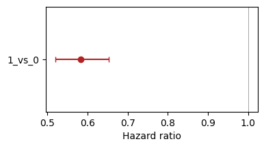
Plot: forest plot of hazard ratios

import matplotlib.pyplot as plt
from pymargins import reference

scen, W = reference("treated", [0, 1], ref_level=0)
res = m.contrasts(scenarios=scen, contrasts=W)
df_forest = res.to_frame()

fig, ax = plt.subplots(figsize=(4, 2))
y = range(len(df_forest))
ax.errorbar(
    df_forest["estimate"], y,
    xerr=[df_forest["estimate"] - df_forest["ci_lower"],
          df_forest["ci_upper"] - df_forest["estimate"]],
    fmt="o", capsize=3, color="firebrick"
)
ax.axvline(1, color="grey", lw=0.5)
ax.set_yticks(list(y))
ax.set_yticklabels(df_forest["label"])
ax.set_xlabel("Hazard ratio")
ax.invert_yaxis()

/home/hunter/.pyenv/versions/3.12.13/lib/python3.12/site-packages/matplotlib/cbook.py:1719: FutureWarning: Calling float on a single element Series is deprecated and will raise a TypeError in the future. Use float(ser.iloc[0]) instead
  return math.isfinite(val)

See Accelerated failure time models for parametric AFT models, where the natural inference scale is the time scale rather than the hazard scale.