Getting started
This tutorial fits a small logit model, opens a Margins session, and
walks through the three orthogonal axes: estimand, aggregation, and
inference. By the end you should be able to map every common
Stata-style margins invocation to its pymargins equivalent.
import numpy as np
import pandas as pd
import statsmodels.api as sm
import statsmodels.formula.api as smf

from pymargins import Margins

rng = np.random.default_rng(0)
n = 4000
df = pd.DataFrame({
    "age": rng.integers(20, 75, n),
    "female": rng.binomial(1, 0.52, n),
    "treated": rng.binomial(1, 0.40, n),
})
lp = -1.5 + 0.04 * df["age"] - 0.3 * df["female"] + 0.8 * df["treated"]
df["y"] = rng.binomial(1, 1 / (1 + np.exp(-lp)))
1. Fit a model
fit = smf.glm(
    "y ~ age + female + treated",
    data=df,
    family=sm.families.Binomial(),
).fit()
print(fit.summary())
                 Generalized Linear Model Regression Results
==============================================================================
Dep. Variable:                      y   No. Observations:                 4000
Model:                            GLM   Df Residuals:                     3996
Model Family:                Binomial   Df Model:                            3
Link Function:                  Logit   Scale:                          1.0000
Method:                          IRLS   Log-Likelihood:                -2452.6
Date:                Sat, 06 Jun 2026   Deviance:                       4905.3
Time:                        16:33:15   Pearson chi2:                 4.01e+03
No. Iterations:                     4   Pseudo R-squ. (CS):             0.1026
Covariance Type:            nonrobust
==============================================================================
                 coef    std err          z      P>|z|      [0.025      0.975]
------------------------------------------------------------------------------
Intercept     -1.3938      0.115    -12.072      0.000      -1.620      -1.168
age            0.0380      0.002     17.055      0.000       0.034       0.042
female        -0.3229      0.069     -4.686      0.000      -0.458      -0.188
treated        0.7100      0.072      9.924      0.000       0.570       0.850
==============================================================================
2. Open a session
A session commits to an inference scale, a vcov estimator, a
confidence level, an aggregation default (at=), and an inference
method. Once constructed, every call inherits these commitments.
m = Margins.log_scale(fit, vcov="HC3", level=0.95, at="overall")
print(m.summary())
Margins session
  Model: GLMResultsWrapper
  Adapter: StatsmodelsGLMAdapter
  Inference scale: log
  Variance: HC3
  Confidence level: 0.95
  At: overall
  Method: delta (κ-threshold=0.3)
  n_sim: 4000
  n_boot: 1000
  Gradient backend: autodiff
  Diagnostics: enabled
  Strict: False
Margins.log_scale(...) is shorthand for
Margins(..., phi=jnp.exp, phi_inv=jnp.log). We use it here because
we will compute a risk-ratio contrast below; for predicted
probabilities linear_scale (identity) or logit_scale are also
valid choices. See Inference scale (phi / phi_inv) for the
full scale menu.
3. Adjusted predictions
Predictions on the response scale, averaged over the observed
distribution of the other covariates (at="overall", the AAP):
print(m.predict(atexog={"treated": [0, 1]}).summary())
===============================================================
               Margins Result (delta, level=0.95)
===============================================================
           estimate  std err         z  P>|z|  [95% Conf. Int.]
---------------------------------------------------------------
treated=0    0.5529   0.0175  -33.7760  0.000    0.5343, 0.5723
treated=1    0.7037   0.0156  -22.4664  0.000    0.6824, 0.7256
===============================================================

n = 4000
Note: std err is on the inference scale; estimate and CI are on the reporting scale.
κ: max=0.038
Delta-vs-sim disagreement: 0.321%
Because the session is on the log scale, the CI is asymmetric on the
probability scale (multiplicative around the point estimate). For a
probability that can approach 1, logit_scale keeps the CI inside
(0, 1); linear_scale gives a symmetric CI on the probability scale
itself.
The same predictions at the typical covariate profile (the APM —
at="typical" uses median for continuous and mode for discrete):
print(Margins.log_scale(fit, vcov="HC3", at="typical").predict(
    atexog={"treated": [0, 1]}
).summary())
===============================================================
               Margins Result (delta, level=0.95)
===============================================================
           estimate  std err         z  P>|z|  [95% Conf. Int.]
---------------------------------------------------------------
treated=0    0.5173   0.0259  -25.4821  0.000    0.4917, 0.5442
treated=1    0.6855   0.0206  -18.2990  0.000    0.6584, 0.7138
===============================================================

n = 4000
Note: std err is on the inference scale; estimate and CI are on the reporting scale.
κ: max=0.045
Delta-vs-sim disagreement: 0.262%
4. Marginal effects
Average marginal effect of age on the response scale:
print(m.dydx("age").summary())
=========================================================
            Margins Result (delta, level=0.95)
=========================================================
     estimate  std err         z  P>|z|  [95% Conf. Int.]
---------------------------------------------------------
age    0.0081   0.0556  -86.6161  0.000    0.0073, 0.0090
=========================================================

n = 4000
Note: std err is on the inference scale; estimate and CI are on the reporting scale.
κ: 0.064
Delta-vs-sim disagreement: 2.688%
A subgroup AME — same call, with female fixed at each level:
print(m.dydx("age", atexog={"female": [0, 1]}).summary())
/home/hunter/Workspace/pymargins/pymargins/margins/_session.py:972: UserWarning: Delta-method curvature κ=0.319 exceeds threshold (0.3, stacklevel=2); falling back to simulation.
  result_data = run_inference(
=========================================================================
                 Margins Result (simulation, level=0.95)
=========================================================================
                    estimate  std err  statistic  P>|z|  [95% Conf. Int.]
-------------------------------------------------------------------------
female=[0, 1], age    0.0081   0.0508    -4.8166  0.000    0.0072, 0.0088
=========================================================================

n = 4000
WARNING — Fallback triggered: kappa=0.319>threshold=0.3
Note: std err is on the inference scale; estimate and CI are on the reporting scale.
κ: 0.319
5. Contrasts
A risk-ratio contrast (treated=1 vs treated=0):
rr = m.contrasts(
    scenarios=[
        {"atexog": {"treated": 1}, "label": "treated"},
        {"atexog": {"treated": 0}, "label": "control"},
    ],
    contrasts=[+1, -1],
)
print(rr.summary())
============================================================
             Margins Result (delta, level=0.95)
============================================================
         estimate  std err        z  P>|z|  [95% Conf. Int.]
------------------------------------------------------------
treated    1.2726   0.0235  10.2554  0.000    1.2153, 1.3326
============================================================

n = 4000
Note: std err is on the inference scale; estimate and CI are on the reporting scale.
κ: 0.025
Delta-vs-sim disagreement: 0.372%
Because the session is on the log scale, the back-transform turns a log-RR into an RR with an asymmetric CI. See Inference scale (phi / phi_inv).
6. Pre-flight diagnostic
print(m.diagnose().summary())
Session diagnostic (50 design points)
  Session: Margins session
  Model: GLMResultsWrapper
  Adapter: StatsmodelsGLMAdapter
  Inference scale: log
  Variance: HC3
  Confidence level: 0.95
  At: overall
  Method: delta (κ-threshold=0.3)
  n_sim: 4000
  n_boot: 1000
  Gradient backend: autodiff
  Diagnostics: enabled
  Strict: False
  κ min:    0.023
  κ median: 0.037
  κ max:    0.082
  Verdict:  delta_reliable
  Delta method is reliable across the design. Spot-check with method='simulation' for estimands at extreme covariate values.
diagnose() computes the κ curvature diagnostic on a sample of the
estimand surface. When κ is small the delta method is reliable; when
κ is large pymargins will auto-fall-back to simulation on the
next call. See The κ curvature diagnostic.
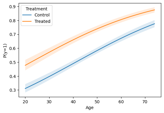
Plot: prediction curve over a continuous variable
import matplotlib.pyplot as plt

ages = list(range(20, 76, 2))
res = m.predict(atexog={"age": ages, "treated": [0, 1]})
df_plot = res.to_frame()

fig, ax = plt.subplots(figsize=(6, 4))
for level, sub in df_plot.groupby("treated"):
    label = "Treated" if level == 1 else "Control"
    ax.plot(sub["age"], sub["estimate"], label=label)
    ax.fill_between(
        sub["age"], sub["ci_lower"], sub["ci_upper"], alpha=0.15
    )
ax.set(xlabel="Age", ylabel="P(y=1)")
ax.legend(title="Treatment")
<matplotlib.legend.Legend at 0x7f050c923da0>
Where to next
GLM — Binomial logit — a deeper logit walkthrough with factor variables.
Contrasts and difference-in-differences — pairwise contrasts and 2×2 DiD.
Inference — delta, simulation, bootstrap — delta vs simulation vs bootstrap.