Spector & Mazzeo (1980) — Did PSI work?
Thirty-two economics students. Three covariates: incoming GPA, a
diagnostic test score (TUCE), and a binary indicator PSI for
whether the student was taught via Personalized System of
Instruction. Outcome GRADE is 1 if the student’s grade improved.
The dataset is tiny — small enough that the uncertainty dominates
the analysis. That makes it perfect for demonstrating how
pymargins lets you cross-check delta-method intervals against a
simulation or bootstrap with one keyword change, and how the κ
diagnostic flags when those methods disagree.
import numpy as np
import pandas as pd
import statsmodels.api as sm
import statsmodels.formula.api as smf

from pymargins import Margins, pairwise

data = sm.datasets.spector.load_pandas()
df = data.exog.copy()
df["GRADE"] = data.endog.astype(int)
print(df.describe().round(2))
         GPA   TUCE    PSI  GRADE
count  32.00  32.00  32.00  32.00
mean    3.12  21.94   0.44   0.34
std     0.47   3.90   0.50   0.48
min     2.06  12.00   0.00   0.00
25%     2.81  19.75   0.00   0.00
50%     3.06  22.50   0.00   0.00
75%     3.51  25.00   1.00   1.00
max     4.00  29.00   1.00   1.00
1. Fit the logit
fit = smf.glm(
    "GRADE ~ GPA + TUCE + PSI",
    data=df,
    family=sm.families.Binomial(),
).fit()
print(fit.summary().tables[1])
==============================================================================
                 coef    std err          z      P>|z|      [0.025      0.975]
------------------------------------------------------------------------------
Intercept    -13.0213      4.931     -2.641      0.008     -22.686      -3.356
GPA            2.8261      1.263      2.238      0.025       0.351       5.301
TUCE           0.0952      0.142      0.672      0.501      -0.182       0.373
PSI            2.3787      1.065      2.234      0.025       0.292       4.465
==============================================================================
2. The treatment effect three ways
The substantive question is “what does PSI do to the probability of grade improvement, holding GPA and TUCE fixed?” That’s a contrast between PSI=1 and PSI=0:
scen, w = pairwise("PSI", [1, 0])

m_delta = Margins.linear_scale(fit, vcov="HC1", at="overall")
print("Delta method:")
print(m_delta.contrasts(scenarios=scen, contrasts=w).summary())
Delta method:
=========================================================
            Margins Result (delta, level=0.95)
=========================================================
       estimate  std err       z  P>|z|  [95% Conf. Int.]
---------------------------------------------------------
PSI=1    0.3575   0.1508  2.3709  0.018    0.0620, 0.6531
=========================================================

n = 32
κ: 0.214
Delta-vs-sim disagreement: 5.604%
With only 32 observations the delta-method CI is wide. A Krinsky–Robb simulation is the cleanest cross-check that does not require refits:
m_sim = Margins.linear_scale(
    fit, vcov="HC1", at="overall",
    method="simulation", n_sim=2000, rng_seed=0,
)
print("Krinsky–Robb simulation:")
print(m_sim.contrasts(scenarios=scen, contrasts=w).summary())
Krinsky–Robb simulation:
============================================================
          Margins Result (simulation, level=0.95)
============================================================
       estimate  std err  statistic  P>|z|  [95% Conf. Int.]
------------------------------------------------------------
PSI=1    0.3575   0.1388     0.3575  0.014    0.0719, 0.6153
============================================================

n = 32
κ: 0.214
A paired bootstrap is the more general non-parametric check, but with n=32 and three covariates the resampled datasets are frequently perfectly separable — the logit refit fails to converge and the bootstrap is not the right tool for this size of problem. The κ diagnostic gives the analytical reason the delta and simulation intervals agree:
print(m_delta.diagnose().summary())
Session diagnostic (32 design points)
  Session: Margins session
  Model: GLMResultsWrapper
  Adapter: StatsmodelsGLMAdapter
  Inference scale: identity
  Variance: HC1
  Confidence level: 0.95
  At: overall
  Method: delta (κ-threshold=0.3)
  n_sim: 4000
  n_boot: 1000
  Gradient backend: autodiff
  Diagnostics: enabled
  Strict: False
  κ min:    0.042
  κ median: 0.632
  κ max:    1.488
  Verdict:  delta_unreliable
  Delta method is unreliable for this analytical posture. Use method='simulation' or method='bootstrap' for inference, or reconsider the inference scale (phi).
A small κ confirms the response surface is essentially linear in the neighborhood being asked about, so the delta method is the cheapest correct answer. A large κ would point you straight at the simulation column.
3. Heterogeneous treatment effect — does PSI help everyone equally?
Compute the PSI vs no-PSI contrast at three representative GPA
levels. This is at doing real work — each row of the result is the
treatment effect at a fixed GPA, with the other covariate (TUCE)
held at its sample average:
gpas = [2.5, 3.0, 3.5]
k = len(gpas)
scenarios = [
    {"atexog": {"PSI": 1, "GPA": g}, "label": f"PSI=1, GPA={g}"} for g in gpas
] + [
    {"atexog": {"PSI": 0, "GPA": g}, "label": f"PSI=0, GPA={g}"} for g in gpas
]
W = np.zeros((k, 2 * k))
for i in range(k):
    W[i, i] = +1.0
    W[i, k + i] = -1.0
het = m_delta.contrasts(scenarios=scenarios, contrasts=W)
print(het.summary())
/home/hunter/Workspace/pymargins/pymargins/margins/_session.py:1213: UserWarning: Delta-method curvature κ=0.712 exceeds threshold (0.3, stacklevel=2); falling back to simulation.
  result_data = run_inference(
==================================================================
             Margins Result (simulation, level=0.95)
==================================================================
             estimate  std err  statistic  P>|z|  [95% Conf. Int.]
------------------------------------------------------------------
contrast[0]    0.1684   0.1506     0.1684  0.015    0.0112, 0.5568
contrast[1]    0.3989   0.1630     0.3989  0.015    0.0675, 0.6903
contrast[2]    0.5190   0.1659     0.5190  0.015    0.1098, 0.7437
==================================================================

n = 32
WARNING — Fallback triggered: kappa=0.712>threshold=0.3
κ: max=0.712
If the joint effect is statistically distinguishable from zero but the individual GPA-stratified effects are not, that’s a signal that the dataset has just enough power for an average claim and not enough for a subgroup claim. With n=32 this happens a lot.
4. Predicted probability curves
import matplotlib.pyplot as plt

gpa_grid = np.linspace(df["GPA"].min(), df["GPA"].max(), 40)
res = m_delta.predict(atexog={"GPA": gpa_grid, "PSI": [0, 1]})
df_plot = res.to_frame()

fig, ax = plt.subplots(figsize=(6, 4))
for psi, sub in df_plot.groupby("PSI"):
    label = "PSI" if psi == 1 else "Control"
    ax.plot(sub["GPA"], sub["estimate"], label=label)
    ax.fill_between(
        sub["GPA"], sub["ci_lower"], sub["ci_upper"], alpha=0.2
    )
ax.set(xlabel="Entering GPA", ylabel="P(grade improvement)")
ax.legend()
/home/hunter/Workspace/pymargins/pymargins/margins/_session.py:875: UserWarning: Delta-method curvature κ=1.771 exceeds threshold (0.3, stacklevel=2); falling back to simulation.
  result_data = run_inference(
<matplotlib.legend.Legend at 0x7fe2401932f0>
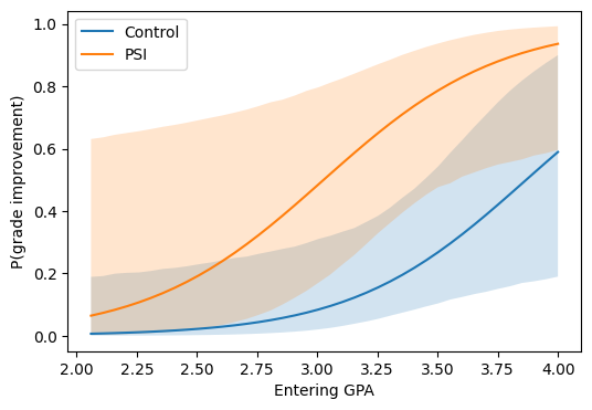
The plot makes the small-sample story honest: the PSI curve sits above the control curve at every GPA, but the CIs overlap heavily, which the contrast table above already told you in scalar form.
Where to next
Inference — delta, simulation, bootstrap — delta vs simulation vs bootstrap, side by side, on a single estimand.
Bootstrap inference — bootstrap recipes.
The κ curvature diagnostic — what κ measures and when it triggers a fallback.