Elasticities and semi-elasticities

import numpy as np
import pandas as pd
import statsmodels.api as sm
import statsmodels.formula.api as smf
from pymargins import Margins

rng = np.random.default_rng(42)
n = 2000
df = pd.DataFrame({
    "x": rng.normal(50, 10, n),
    "female": rng.binomial(1, 0.52, n),
})
lp = -1.5 + 0.03 * df["x"] - 0.3 * df["female"]
df["y"] = rng.binomial(1, 1 / (1 + np.exp(-lp)))

fit = smf.glm("y ~ x + female", data=df,
              family=sm.families.Binomial()).fit()
m = Margins.linear_scale(fit, at="overall")

dydx returns the level derivative. The three elasticity / semi-elasticity flavours are available directly as session methods:

Stata margins	Quantity	pymargins method
dydx(x)	level change	m.dydx("x")
dyex(x)	dy/d(ln x)	m.dyex("x")
eyex(x)	full elasticity (dy/dx) (x/y)	m.eyex("x")
eydx(x)	d(ln y)/dx	m.eydx("x")

Each method computes the slope and prediction internally and composes them with the correct transform, carrying the joint gradient through the delta method so standard errors and confidence intervals are valid.

Basic usage

# Full elasticity at the session's `at` setting
print(m.eyex("x").summary())

# Semi-elasticities
print(m.eydx("x").summary())
print(m.dyex("x").summary())

===========================================================
             Margins Result (delta, level=0.95)            
===========================================================
         estimate  std err       z  P>|z|  [95% Conf. Int.]
-----------------------------------------------------------
eyex(x)    0.8661   0.1357  6.3829  0.000    0.6001, 1.1320
===========================================================

n = 2000
κ: 0.033
===========================================================
             Margins Result (delta, level=0.95)            
===========================================================
         estimate  std err       z  P>|z|  [95% Conf. Int.]
-----------------------------------------------------------
eydx(x)    0.0175   0.0027  6.3829  0.000    0.0121, 0.0229
===========================================================

n = 2000
κ: 0.033

===========================================================
             Margins Result (delta, level=0.95)            
===========================================================
         estimate  std err       z  P>|z|  [95% Conf. Int.]
-----------------------------------------------------------
dyex(x)    0.3858   0.0597  6.4625  0.000    0.2688, 0.5028
===========================================================

n = 2000
κ: 0.033

These methods honour atexog and over just like dydx:

# Elasticity of x within each level of female
print(m.eyex("x", over="female").summary())

============================================================
             Margins Result (delta, level=0.95)             
============================================================
         estimate  std err        z  P>|z|  [95% Conf. Int.]
------------------------------------------------------------
eyex(x)    0.7960   1.9877   0.4004  0.689   -3.0999, 4.6918
[1]        0.9429   0.0351  26.8567  0.000    0.8741, 1.0117
============================================================

n = 2000
κ: max=0.025

Under the hood: manual composition with .scaled()

If you need a custom scaling factor (e.g. a subgroup mean that is not the overall mean, or a theoretical value), the underlying recipe is a compose_results of the slope and prediction. The convenience methods above are exactly this pattern wrapped for you.

For reference, eyex is equivalent to:

from pymargins._result._margins import compose_results
import jax.numpy as jnp

slope_x = m.dydx("x")
pred    = m.predict()
x_bar   = float(df["x"].mean())

elasticity = compose_results(
    [slope_x, pred],
    fn=lambda t: t[0] * x_bar / t[1],
    label="eyex(x)",
)

The .scaled(by=...) helper offers a lighter-weight alternative when the scaling factor is a simple scalar:

x_bar = df["x"].mean()
y_bar = m.predict().estimate.item()

# eyex via scaled()
print(m.dydx("x").scaled(by=x_bar / y_bar).summary())

=========================================================================
                    Margins Result (delta, level=0.95)                   
=========================================================================
                       estimate  std err       z  P>|z|  [95% Conf. Int.]
-------------------------------------------------------------------------
(x)*110.9958295306184    0.8661   0.1340  6.4625  0.000    0.6034, 1.1287
=========================================================================

n = 2000
κ: 0.033
Delta-vs-sim disagreement: 3.991%

scaled is a deterministic transform — it propagates SE, CI, and covariance correctly under the delta method.

Subgroup elasticities

Because .scaled() propagates the joint covariance, you can compute elasticities for several subgroups and test differences between them:

# Subgroup means for scaling
x_bar_0 = df.loc[df["female"] == 0, "x"].mean()
y_bar_0 = m.predict(atexog={"female": 0}).estimate.item()
x_bar_1 = df.loc[df["female"] == 1, "x"].mean()
y_bar_1 = m.predict(atexog={"female": 1}).estimate.item()

# Elasticity of x for female=0 and female=1
res_0 = m.dydx("x", atexog={"female": 0}).scaled(by=x_bar_0 / y_bar_0)
res_1 = m.dydx("x", atexog={"female": 1}).scaled(by=x_bar_1 / y_bar_1)

# Difference in elasticities with a proper SE
diff = res_1 - res_0
print(diff.summary())

==========================================================================================================================
                                            Margins Result (delta, level=0.95)                                            
==========================================================================================================================
                                                                        estimate  std err       z  P>|z|  [95% Conf. Int.]
--------------------------------------------------------------------------------------------------------------------------
((female=1, x)*124.31135122094987) - ((female=0, x)*98.94062025641874)    0.1627   0.0177  9.1912  0.000    0.1280, 0.1974
==========================================================================================================================

n = 2000
κ: 0.037

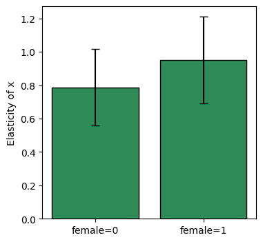
Plot: comparing elasticities across subgroups

import matplotlib.pyplot as plt

df_0 = res_0.to_frame()
df_1 = res_1.to_frame()

labels = ["female=0", "female=1"]
estimates = [df_0["estimate"].iloc[0], df_1["estimate"].iloc[0]]
ci_lower = [df_0["ci_lower"].iloc[0], df_1["ci_lower"].iloc[0]]
ci_upper = [df_0["ci_upper"].iloc[0], df_1["ci_upper"].iloc[0]]

fig, ax = plt.subplots(figsize=(4, 4))
ax.bar(labels, estimates,
       yerr=[np.array(estimates) - np.array(ci_lower),
             np.array(ci_upper) - np.array(estimates)],
       capsize=4, color="seagreen", edgecolor="black")
ax.set(ylabel="Elasticity of x")

[Text(0, 0.5, 'Elasticity of x')]

Pitfalls

• Division by near-zero predictions. Elasticities blow up when the predicted response is close to zero. The convenience methods clip near-zero denominators at 1e-12 by default; for a more principled solution, consider a log-scale session (Margins.log_scale(...)) which linearises the problem.

• Discrete inputs. Elasticities are only defined for continuous variables — pymargins raises on discrete inputs.