Fair (1978) — Extramarital affairs, two ways
The Fair affairs survey records the number of extramarital encounters reported by 6,366 respondents, alongside age, years married, religiousness, education, and a marriage-rating scale. The same dataset supports two distinct analyses:
a logit on
had_affair = affairs > 0— the binary question, “is this respondent at risk of any affair at all?”a Poisson on
affairsitself — the count question, “how many encounters do we expect from a respondent at this profile?”
Both are useful. The point of this demo is to run them through one
pymargins session each and contrast how they answer the same
substantive questions on different scales.
import numpy as np
import pandas as pd
import statsmodels.api as sm
import statsmodels.formula.api as smf

from pymargins import Margins, pairwise

raw = sm.datasets.fair.load_pandas().data.copy()
raw["had_affair"] = (raw["affairs"] > 0).astype(int)
print(raw[["had_affair", "affairs", "age", "yrs_married",
           "religious", "rate_marriage"]].describe().round(2))
       had_affair  affairs      age  yrs_married  religious  rate_marriage
count     6366.00  6366.00  6366.00      6366.00    6366.00        6366.00
mean         0.32     0.71    29.08         9.01       2.43           4.11
std          0.47     2.20     6.85         7.28       0.88           0.96
min          0.00     0.00    17.50         0.50       1.00           1.00
25%          0.00     0.00    22.00         2.50       2.00           4.00
50%          0.00     0.00    27.00         6.00       2.00           4.00
75%          1.00     0.48    32.00        16.50       3.00           5.00
max          1.00    57.60    42.00        23.00       4.00           5.00
1. Logit on the binary outcome
logit = smf.glm(
    "had_affair ~ age + yrs_married + religious + rate_marriage + educ",
    data=raw,
    family=sm.families.Binomial(),
).fit()

m_logit = Margins.linear_scale(logit, vcov="HC3", at="overall")
print(m_logit.dydx(["age", "yrs_married", "religious",
                    "rate_marriage", "educ"]).summary())
===================================================================
                 Margins Result (delta, level=0.95)
===================================================================
               estimate  std err         z  P>|z|  [95% Conf. Int.]
-------------------------------------------------------------------
age             -0.0107   0.0018   -5.8172  0.000  -0.0143, -0.0071
yrs_married      0.0196   0.0017   11.8120  0.000    0.0164, 0.0229
religious       -0.0679   0.0063  -10.8099  0.000  -0.0802, -0.0556
rate_marriage   -0.1275   0.0066  -19.4033  0.000  -0.1404, -0.1146
educ            -0.0021   0.0026   -0.7967  0.426   -0.0073, 0.0031
===================================================================

n = 6366
κ: max=0.084
Delta-vs-sim disagreement: 16.593%
The AMEs are reported as changes in the probability of any affair per unit of each covariate, averaged over the observed sample. The signs match intuition: longer marriages and lower marriage ratings raise the probability, religiousness lowers it.
2. Poisson on the count
pois = smf.glm(
    "affairs ~ age + yrs_married + religious + rate_marriage + educ",
    data=raw,
    family=sm.families.Poisson(),
).fit()

m_pois = Margins.linear_scale(pois, vcov="HC3", at="overall")
print(m_pois.dydx(["age", "yrs_married", "religious",
                   "rate_marriage", "educ"]).summary())
/home/hunter/Workspace/pymargins/pymargins/margins/_session.py:972: UserWarning: Delta-method curvature κ=0.602 exceeds threshold (0.3, stacklevel=2); falling back to simulation.
  result_data = run_inference(
====================================================================
              Margins Result (simulation, level=0.95)
====================================================================
               estimate  std err  statistic  P>|z|  [95% Conf. Int.]
--------------------------------------------------------------------
age             -0.0155   0.0097    -0.0155  0.117   -0.0341, 0.0039
yrs_married     -0.0281   0.0116    -0.0281  0.017  -0.0432, -0.0020
religious       -0.2573   0.0369    -0.2573  0.000  -0.3372, -0.1933
rate_marriage   -0.3511   0.0257    -0.3511  0.000  -0.4054, -0.3044
educ            -0.0070   0.0119    -0.0070  0.557   -0.0305, 0.0162
====================================================================

n = 6366
WARNING — Fallback triggered: kappa=0.602>threshold=0.3
κ: max=0.602
These AMEs are the change in the expected count per unit. The ranking of effects is similar to the logit; the magnitudes are not comparable because they live on different response scales.
3. Marriage rating as a discrete contrast
rate_marriage is recorded on a 1–5 ordinal scale. The natural
policy question is “what’s the gap between a ‘very happy’ marriage
(5) and a ‘very unhappy’ marriage (1)?” — a contrast, not a slope:
scen, w = pairwise("rate_marriage", [5, 1])
print("Logit (probability scale):")
print(m_logit.contrasts(scenarios=scen, contrasts=w).summary())
print("\nPoisson (count scale):")
print(m_pois.contrasts(scenarios=scen, contrasts=w).summary())
Logit (probability scale):
=====================================================================
                  Margins Result (delta, level=0.95)
=====================================================================
                 estimate  std err         z  P>|z|  [95% Conf. Int.]
---------------------------------------------------------------------
rate_marriage=5   -0.5819   0.0209  -27.8855  0.000  -0.6228, -0.5410
=====================================================================

n = 6366
κ: 0.043
Delta-vs-sim disagreement: 0.607%

Poisson (count scale):
====================================================================
                 Margins Result (delta, level=0.95)
====================================================================
                 estimate  std err        z  P>|z|  [95% Conf. Int.]
--------------------------------------------------------------------
rate_marriage=5   -2.5910   0.2767  -9.3637  0.000  -3.1333, -2.0486
====================================================================

n = 6366
κ: 0.089
Delta-vs-sim disagreement: 2.798%
The logit contrast says: averaging across the sample, a respondent rating their marriage 5 has X percentage points lower probability of any affair than the same respondent at rating 1. The Poisson contrast gives the corresponding gap in expected count.
4. Scale matters — log vs linear inference for the Poisson
The Poisson canonical link is log. Opening the session on the log scale gives a rate ratio interpretation with an asymmetric CI that is multiplicative on the count scale, which is usually what readers expect for count models:
m_pois_log = Margins.log_scale(pois, vcov="HC3", at="overall")
rr = m_pois_log.contrasts(scenarios=scen, contrasts=w)
print(rr.summary())
=====================================================================
                  Margins Result (delta, level=0.95)
=====================================================================
                 estimate  std err         z  P>|z|  [95% Conf. Int.]
---------------------------------------------------------------------
rate_marriage=5    0.1336   0.1240  -16.2310  0.000    0.1048, 0.1704
=====================================================================

n = 6366
Note: std err is on the inference scale; estimate and CI are on the reporting scale.
κ: 0.000
Delta-vs-sim disagreement: 1.815%
The point estimate here is log(rate ratio); the back-transformed CI is the rate ratio with an asymmetric interval. See Inference scale (phi / phi_inv) for the menu of scales.
The κ diagnostic checks whether the estimand surface is well linearized on the chosen scale:
print(m_pois_log.diagnose().summary())
Session diagnostic (50 design points)
  Session: Margins session
  Model: GLMResultsWrapper
  Adapter: StatsmodelsGLMAdapter
  Inference scale: log
  Variance: HC3
  Confidence level: 0.95
  At: overall
  Method: delta (κ-threshold=0.3)
  n_sim: 4000
  n_boot: 1000
  Gradient backend: autodiff
  Diagnostics: enabled
  Strict: False
  κ min:    0.000
  κ median: 0.000
  κ max:    0.000
  Verdict:  delta_reliable
  Delta method is reliable across the design. Spot-check with method='simulation' for estimands at extreme covariate values.
A small κ confirms the delta method is safe on the log scale; a large κ would trigger an automatic fallback to simulation.
5. Predicted profile over years married
import matplotlib.pyplot as plt

years = list(range(0, 25))
res_l = m_logit.predict(atexog={"yrs_married": years})
res_p = m_pois.predict(atexog={"yrs_married": years})

fig, axes = plt.subplots(1, 2, figsize=(10, 4), sharex=True)
for ax, res, ylabel in [
    (axes[0], res_l, "P(any affair)"),
    (axes[1], res_p, "E(affairs)"),
]:
    d = res.to_frame()
    ax.plot(d["yrs_married"], d["estimate"], color="firebrick")
    ax.fill_between(
        d["yrs_married"], d["ci_lower"], d["ci_upper"],
        alpha=0.2, color="firebrick",
    )
    ax.set(xlabel="Years married", ylabel=ylabel)
fig.suptitle("Same dataset, two estimands")
fig.tight_layout()
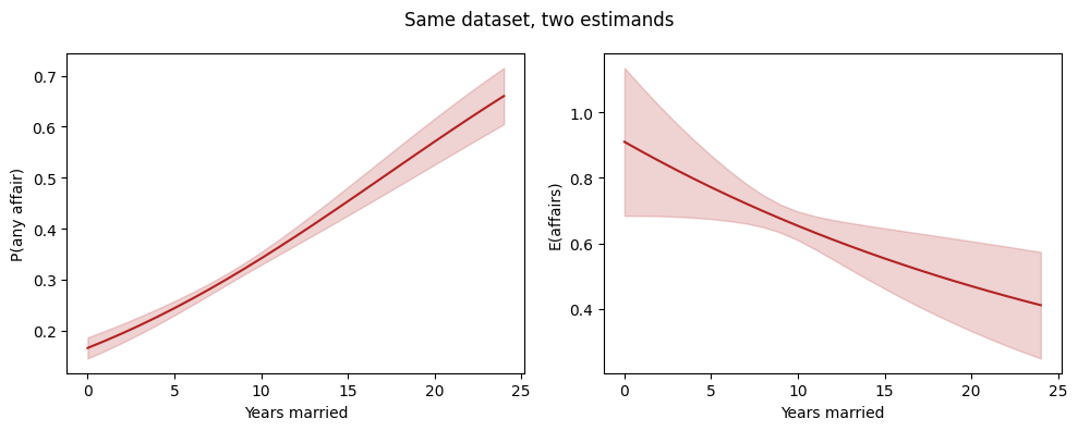
The shapes are similar but not identical — the logit saturates as
yrs_married grows, the Poisson does not. Which curve to report
depends on whether the audience cares about who has affairs or
how many.
Where to next
GLM — Poisson count — Poisson tutorial with offsets.
Inference scale (phi / phi_inv) — log vs linear vs logit scale and what each one buys you.
Mroz (1987) — Female labor force participation — same model family, focused on the AME-vs-MEM question.