Generalised Estimating Equations (GEE)

statsmodels.GEE handles correlated outcomes through a working correlation structure and sandwich covariance. pymargins consumes the GEE fit directly — the robust (sandwich) covariance is the default, and the session API is identical to GLM.

import numpy as np
import pandas as pd
import statsmodels.api as sm
import statsmodels.formula.api as smf

from pymargins import Margins

rng = np.random.default_rng(42)
n = 600
df = pd.DataFrame({
    "age": rng.integers(20, 75, n),
    "female": rng.binomial(1, 0.52, n),
    "treated": rng.binomial(1, 0.40, n),
    "site": rng.choice(["A", "B", "C", "D"], n),
    "subject": np.repeat(np.arange(60), 10),
})
lp = -1.5 + 0.04 * df["age"] - 0.3 * df["female"] + 0.8 * df["treated"]
df["y"] = rng.binomial(1, 1 / (1 + np.exp(-lp)))

fit = smf.gee(
    "y ~ age + female + treated + C(site)",
    groups="subject",
    data=df,
    family=sm.families.Binomial(),
    cov_struct=sm.cov_struct.Independence(),
).fit()

Average marginal effect of age

The default covariance is the GEE sandwich (robust) estimator:

m = Margins.linear_scale(fit, at="overall")
print(m.dydx("age").summary())

=======================================================
           Margins Result (delta, level=0.95)          
=======================================================
     estimate  std err       z  P>|z|  [95% Conf. Int.]
-------------------------------------------------------
age    0.0095   0.0016  6.0065  0.000    0.0064, 0.0126
=======================================================

n = 600
κ: 0.073
Delta-vs-sim disagreement: 12.145%

Predicted probabilities by treatment arm

print(m.predict(atexog={"treated": [0, 1]}).summary())

==============================================================
              Margins Result (delta, level=0.95)              
==============================================================
           estimate  std err        z  P>|z|  [95% Conf. Int.]
--------------------------------------------------------------
treated=0    0.5450   0.0201  27.1783  0.000    0.5057, 0.5843
treated=1    0.7111   0.0295  24.1027  0.000    0.6533, 0.7689
==============================================================

n = 600
κ: max=0.062
Delta-vs-sim disagreement: 0.844%

Risk difference for treatment

from pymargins import pairwise

scen, w = pairwise("treated", [1, 0])
print(m.contrasts(scenarios=scen, contrasts=w).summary())

=============================================================
              Margins Result (delta, level=0.95)             
=============================================================
           estimate  std err       z  P>|z|  [95% Conf. Int.]
-------------------------------------------------------------
treated=1    0.1661   0.0374  4.4473  0.000    0.0929, 0.2393
=============================================================

n = 600
κ: 0.053
Delta-vs-sim disagreement: 2.091%

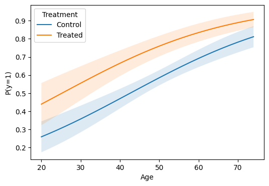
Plot: predicted probability curve over age

import matplotlib.pyplot as plt

ages = list(range(20, 76, 2))
res = m.predict(atexog={"age": ages, "treated": [0, 1]})
df_plot = res.to_frame()

fig, ax = plt.subplots(figsize=(6, 4))
for level, sub in df_plot.groupby("treated"):
    label = "Treated" if level == 1 else "Control"
    ax.plot(sub["age"], sub["estimate"], label=label)
    ax.fill_between(
        sub["age"], sub["ci_lower"], sub["ci_upper"], alpha=0.15
    )
ax.set(xlabel="Age", ylabel="P(y=1)")
ax.legend(title="Treatment")

<matplotlib.legend.Legend at 0x7f678c8dc500>

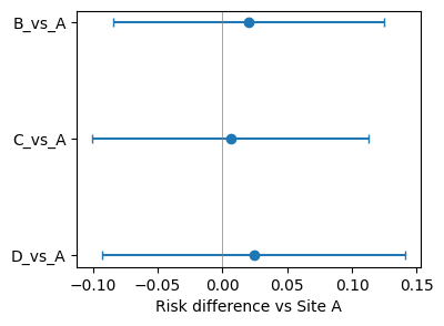
Plot: forest plot of site contrasts

from pymargins import reference

scen, W = reference("site", ["A", "B", "C", "D"], ref_level="A")
res = m.contrasts(scenarios=scen, contrasts=W)
df_forest = res.to_frame()

fig, ax = plt.subplots(figsize=(4, 3))
y = range(len(df_forest))
ax.errorbar(
    df_forest["estimate"], y,
    xerr=[df_forest["estimate"] - df_forest["ci_lower"],
          df_forest["ci_upper"] - df_forest["estimate"]],
    fmt="o", capsize=3,
)
ax.axvline(0, color="grey", lw=0.5)
ax.set_yticks(list(y))
ax.set_yticklabels(df_forest["label"])
ax.set_xlabel("Risk difference vs Site A")
ax.invert_yaxis()

Alternative vcov flavours

GEE fits carry three built-in covariances. You can switch at session construction:

# Naive (model-based) covariance
m_naive = Margins.linear_scale(fit, vcov="naive", at="overall")
print(m_naive.dydx("age").summary())

# Bias-corrected robust sandwich (if available)
try:
    m_bc = Margins.linear_scale(fit, vcov="robust_bc", at="overall")
    print(m_bc.dydx("age").summary())
except ValueError as exc:
    print("robust_bc not available:", exc)

=======================================================
           Margins Result (delta, level=0.95)          
=======================================================
     estimate  std err       z  P>|z|  [95% Conf. Int.]
-------------------------------------------------------
age    0.0095   0.0013  7.1816  0.000    0.0069, 0.0121
=======================================================

n = 600
κ: 0.063
Delta-vs-sim disagreement: 9.631%
robust_bc not available: cov_robust_bc is not available on this fit.

Formula vs array interface

If you fit with sm.GEE(y, X, groups=...) instead of smf.gee(...), provide the training data explicitly so the adapter can reconstruct the design matrix:

from pymargins.adapters import StatsmodelsGEEAdapter

adapter = StatsmodelsGEEAdapter(fit_array, training_data=df)
m = Margins.linear_scale(fit_array, adapter=adapter, at="overall")