Inference — delta, simulation, bootstrap

pymargins exposes three inference paths behind one session keyword, method=. Picking the right one is a function of curvature (κ) and the resampling structure of your data.

import numpy as np
import pandas as pd
import statsmodels.api as sm
import statsmodels.formula.api as smf

from pymargins import Margins

rng = np.random.default_rng(0)
n = 1500
df = pd.DataFrame({
    "x": rng.normal(0, 1, n),
    "g": rng.integers(0, 50, n),
})
lp = -2.5 + 1.6 * df["x"]
df["y"] = rng.binomial(1, 1 / (1 + np.exp(-lp)))

fit = smf.glm("y ~ x", data=df, family=sm.families.Binomial()).fit()

Delta — the default

m = Margins.log_scale(fit, at="overall", method="delta")
print(m.predict(atexog={"x": [-2, 0, 2]}).summary())

==========================================================
            Margins Result (delta, level=0.95)            
==========================================================
      estimate  std err         z  P>|z|  [95% Conf. Int.]
----------------------------------------------------------
x=-2    0.0029   0.3350  -17.4381  0.000    0.0015, 0.0056
x=0     0.0665   0.1175  -23.0812  0.000    0.0528, 0.0837
x=2     0.6350   0.0614   -7.3963  0.000    0.5630, 0.7162
==========================================================

n = 1500
Note: std err is on the inference scale; estimate and CI are on the reporting scale.
κ: max=0.107
Delta-vs-sim disagreement: 13.066%

Krinsky–Robb simulation

Useful when a probability sits near 0 or 1 and the symmetric Wald CI would cross the boundary.

m_sim = Margins.log_scale(fit, at="overall", method="simulation", n_sim=2000)
print(m_sim.predict(atexog={"x": [-2, 0, 2]}).summary())

===========================================================
          Margins Result (simulation, level=0.95)          
===========================================================
      estimate  std err  statistic  P>|z|  [95% Conf. Int.]
-----------------------------------------------------------
x=-2    0.0029   0.3336    -5.8416  0.000    0.0014, 0.0053
x=0     0.0665   0.1162    -2.7112  0.000    0.0523, 0.0825
x=2     0.6350   0.0630    -0.4541  0.000    0.5553, 0.7081
===========================================================

n = 1500
Note: std err is on the inference scale; estimate and CI are on the reporting scale.
κ: max=0.107

Pairs bootstrap

m_boot = Margins.log_scale(
    fit, at="overall", method="bootstrap", n_boot=200
)
print(m_boot.predict(atexog={"x": [-2, 0, 2]}).summary())

===========================================================
           Margins Result (bootstrap, level=0.95)          
===========================================================
      estimate  std err  statistic  P>|z|  [95% Conf. Int.]
-----------------------------------------------------------
x=-2    0.0029   0.3047    -5.8416  0.000    0.0016, 0.0050
x=0     0.0665   0.1103    -2.7112  0.000    0.0529, 0.0818
x=2     0.6350   0.0634    -0.4541  0.000    0.5545, 0.7122
===========================================================

n = 1500
Note: std err is on the inference scale; estimate and CI are on the reporting scale.
κ: max=0.107

Cluster bootstrap

Pass cluster IDs at session construction to switch from pairs to cluster resampling — required when within-cluster correlation matters.

m_clust = Margins.log_scale(
    fit, at="overall", method="bootstrap",
    n_boot=500, cluster=df["g"].values,
)
print(m_clust.predict(atexog={"x": [-2, 0, 2]}).summary())

===========================================================
           Margins Result (bootstrap, level=0.95)          
===========================================================
      estimate  std err  statistic  P>|z|  [95% Conf. Int.]
-----------------------------------------------------------
x=-2    0.0029   0.3057    -5.8416  0.000    0.0016, 0.0049
x=0     0.0665   0.1083    -2.7112  0.000    0.0533, 0.0818
x=2     0.6350   0.0590    -0.4541  0.000    0.5669, 0.7089
===========================================================

n = 1500
Note: std err is on the inference scale; estimate and CI are on the reporting scale.
κ: max=0.107

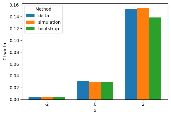
Plot: comparing CI widths across methods

import matplotlib.pyplot as plt

x_grid = [-2, 0, 2]
res_delta = m.predict(atexog={"x": x_grid}).to_frame()
res_sim = m_sim.predict(atexog={"x": x_grid}).to_frame()
res_boot = m_boot.predict(atexog={"x": x_grid}).to_frame()

fig, ax = plt.subplots(figsize=(6, 4))
widths = {
    "delta": res_delta["ci_upper"] - res_delta["ci_lower"],
    "simulation": res_sim["ci_upper"] - res_sim["ci_lower"],
    "bootstrap": res_boot["ci_upper"] - res_boot["ci_lower"],
}
x_pos = np.arange(len(x_grid))
width = 0.25
for i, (label, w) in enumerate(widths.items()):
    ax.bar(x_pos + i * width, w, width, label=label)
ax.set_xticks(x_pos + width)
ax.set_xticklabels([str(v) for v in x_grid])
ax.set(xlabel="x", ylabel="CI width")
ax.legend(title="Method")

<matplotlib.legend.Legend at 0x7ff041b2f2c0>

See Delta vs simulation vs bootstrap for the decision rule.